【数学】基本代数图论 Basic Algebraic Graph Theory

---

1. Notations

• $\mathcal{G}$：图
• $\mathcal{V}$：节点的集合
• $\mathcal{E}$：边的集合
• $\mathcal{A}$：邻接矩阵
• $\mathcal{L}$：拉普拉斯矩阵
• ${\mathcal{N}}_i$：智能体$i$的邻居节点集合

2. Basic Concepts

2.1 Basic Representation of Graph

• 有向图 dircted graph：$\mathcal{G}\triangleq (\mathcal{V},\mathcal{E})$，其中 V ≜ { 1 , … , p } \mathscr{V}\triangleq{\{1,\dots,p\}} V≜{1,…,p}表示节点的集合，$\mathcal{E}\subseteq (\mathcal{V}\times \mathcal{V})$表示边的集合。
• 有向图的边 edge：$(i,j)$表示$j$可以从$i$获取信息，但反过来则不行，且有$(i,j)\in \mathcal{E}$，其中$i$是父节点$j$是子节点。
• 无向图的边 edge：$(i,j)$表示$i$和$j$可以交换信息，无向图的边可以视作是一种特殊的有向图的边，比如无向图的边$(i,j)$可以视作有向图的边$(i,j)$和$(j,i)$的组合。
• 有权图 weighted graph：图中的每一条边都具有权重，如果没有特殊说明，基本所有的图都是有权图。
• 图集合的并 union of a collection of graphs：图集合的并是指，图的节点集合的并和图的边集合的并。
• 邻居节点集合${\mathcal{N}}_i$：代表了所有与智能体$i$具有一条边相连的所有其他智能体构成的集合。

2.2 Basic Relations of Graph

• 有向通路 directed path：是针对有向图而言的，可以用一系列的边来表示$(i_1,i_2),(i_2,i_3)$
• 无向通路 undirected path：是针对无向图而言的，用类似于有向通路的方式来定义。
• 强连接 strongly connected：是针对有向图而言的，$\forall$节点间都$\exists$一条有向通路
• 连接 connected：是针对无向图而言的，$\forall$互异节点间都$\exists$一条无向通路
• 完全 complete：是针对有向图而言的，$\forall$节点间都$\exists$一条边
• 全连接 fully connected：是针对无向图而言的，$\forall$互异节点间都$\exists$一条边
• 有向树 directed tree：是针对于有向图而言的，除了根节点外每个节点都只有一个父节点，而根节点则没有父节点
• 树 tree：是针对于无向图而言的，每一对节点都只由一条无向通路连接。

2.3 Subgraph of Graph

• 子图 subgraph：$({\mathcal{V}}^s,{\mathcal{E}}^s)$是$(\mathcal{V},\mathcal{E})$的子图，其中${\mathcal{V}}^s\subseteq \mathcal{V},{\mathcal{E}}^s\subseteq \mathcal{E}\bigcap ({\mathcal{V}}^s,{\mathcal{V}}^s)$
• 有向生成树 directed spanning tree：$({\mathcal{V}}^s,{\mathcal{E}}^s)$是$(\mathcal{V},\mathcal{E})$的子图，$s.t.$$({\mathcal{V}}^s,{\mathcal{E}}^s)$是有向树，并且${\mathcal{V}}^s=\mathcal{V}$，即子图包含原图的所有节点
• 无向生成树 undirected spanning tree：$({\mathcal{V}}^s,{\mathcal{E}}^s)$是$(\mathcal{V},\mathcal{E})$的子图，$s.t.$$({\mathcal{V}}^s,{\mathcal{E}}^s)$是树，并且${\mathcal{V}}^s=\mathcal{V}$，即子图包含原图的所有节点
• 有向生成树的存在性 existence of directed spanning tree：当有向生成树是图$(\mathcal{V},\mathcal{E})$的子图的时候，我们称图$(\mathcal{V},\mathcal{E})$具有生成树。判据：图$(\mathcal{V},\mathcal{E})$具有生成树$iff$图$(\mathcal{V},\mathcal{E})$至少具有一个节点对其他所有的节点具有有向通路。
• 无向图生成树的存在性 existence of undirected spanning tree：无向图生成树的存在性等同于连接性。

2.4 Adjacency Matrix

• 有向图的邻接矩阵 adjacency matrix of direceted graph：不允许有自边self-edge的图$(\mathcal{V},\mathcal{E})$的邻接矩阵可以表示为$\mathcal{A}\triangleq [a_{ij}]\in {\mathbb{R}}^{p\times p}$，

$$a_{ij}=\{\begin{array}{l}\begin{array}{rlr}& \text{positive weight}& \text{if(j,i)∈E}\\ & 0& \text{if(j,i)∈/E}\\ & 0& \text{ifi=j}\end{array}\end{array}$$

• 无向图的邻接矩阵 adjacency matrix of undirected graph：无向图的邻接矩阵定义类似，只不过多了一条性质是$a_{ij}=a_{ji},i\ne j$，保证了无向图的邻接矩阵是对称的。
• 节点的入度 in-degree：对节点$i$来说，其入度是${\sum }_{j=1}^p{a}_{ij}$
• 节点的出度out-degree：对节点$i$来说，其出度是${\sum }_{j=1}^p{a}_{ji}$
• 平衡点 balanced node：对于节点$i$来说，如果它的入度等于出度，那么它是平衡点。
• 平衡图 balanced graph：对于图来说，如果它的所有结点都是平衡点那么该图则是平衡图。

2.5 Laplacian Matrix

拉普拉斯矩阵 Laplacian Matrix的定义是$\mathcal{L}\triangleq [{\ell }_{ij}]\in {\mathbb{R}}^{p\times p}$
$${\ell }_{ii}=\sum _{j=1,i\ne j}^p{a}_{ij},{\ell }_{ij}=-a_{ij},i\ne j$$
并且注意到$(j,i)\notin \mathcal{E}$则有${\ell }_{ij}=-a_{ij}=0$，那么拉普拉斯矩阵满足：
$${\ell }_{ij}\le 0,i\ne j,\sum _{j=1}^p{\ell }_{ij}=0,i=1,\dots ,p$$

• 无向图的拉普拉斯矩阵是对称阵，直接称为Laplacian matrix
• 有向图的拉普拉斯矩阵是非对称阵，称为nonsymetric Laplacian matrix或者directed Laplacian matrix

入度矩阵in-degree matrix $D\triangleq [d_{ij}]\in {\mathbb{R}}^{p\times p}$的定义是：
$$d_{ij}=\{\begin{array}{l}\begin{array}{rlr}& 0& \text{if i=j}\\ & \sum _{j=1}^p{a}_{ij}& i=1,\dots ,p\end{array}\end{array}$$
那么拉普拉斯矩阵$\mathcal{L}$就可以通过入度矩阵$D$和邻接矩阵$\mathcal{A}$来进行表示
$$\mathcal{L}=D-\mathcal{A}$$

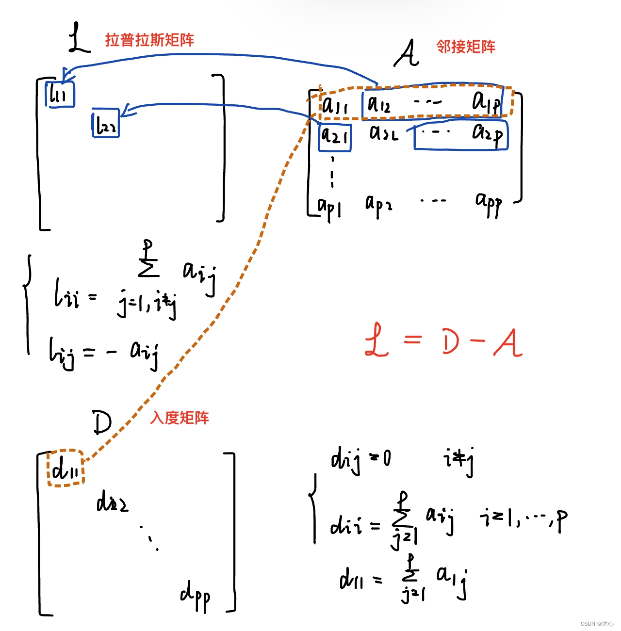
三者基本的关系可以由上图表示。

---

Reference

Distributed Coordination of Multi-agent Networks Emergent Problems, Models, and Issues